Seminar 7: Continuous Random Variables. Normal Distribution

A discrete random variable assigns positive probability to countably many values.

A continuous random variable distributes its probability over intervals rather than individual points. In this lecture we study the most important class of continuous distributions: absolutely continuous distributions.

1 Probability Distributions

A probability distribution on \(\mathbb R\) is a probability measure

\[ P:\mathcal B(\mathbb R)\rightarrow[0,1], \]

where \(\mathcal B(\mathbb R)\) denotes the Borel \(\sigma\)-algebra.

1.1 Cumulative Distribution Function

The cumulative distribution function (CDF) of a random variable \(\xi\) is defined by

\[ F_{\xi}(x)=P(\xi\le x),\qquad x\in\mathbb R. \]

Notice that the CDF completely determines the probability distribution.

In other words, if two random variables have the same cumulative distribution function, then they have the same distribution.

1.1.1 Properties of the CDF

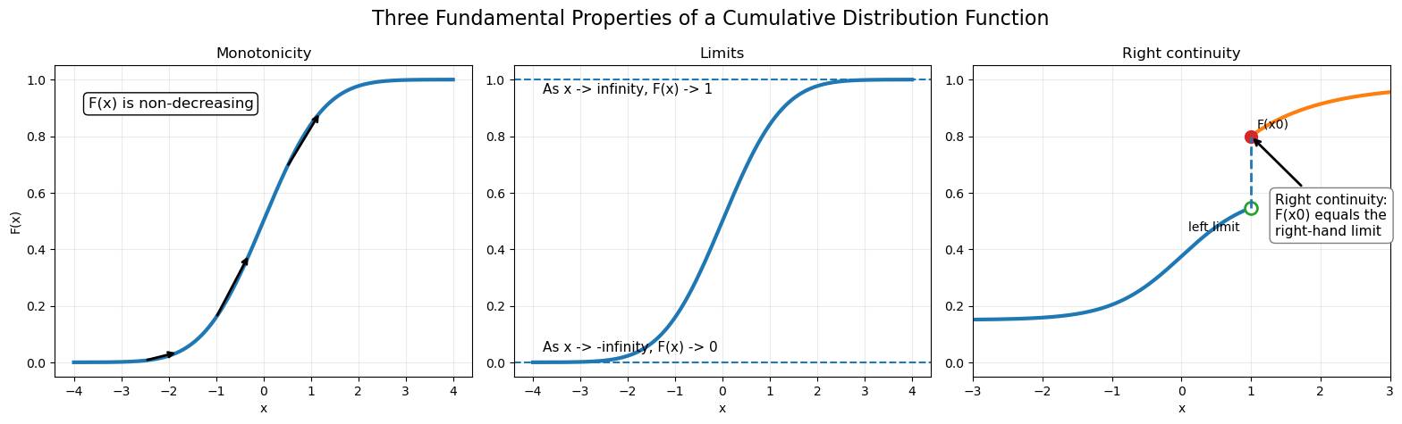
1. \(F(x)\) is non-decreasing.
2. \(\displaystyle\lim_{x\to-\infty}F(x)=0\) and \(\displaystyle\lim_{x\to\infty}F(x)=1\).
3. \(F(x)\) is right-continuous.

import numpy as np
import matplotlib.pyplot as plt
from scipy.stats import norm

x = np.linspace(-4, 4, 1000)
F = norm.cdf(x)

fig, axes = plt.subplots(1, 3, figsize=(16, 4.8))

# =====================================================
# (1) Monotonicity
# =====================================================

ax = axes[0]

ax.plot(x, F, linewidth=3)
ax.set_title("Monotonicity")

for x0 in [-2.5, -1, 0.5]:
    ax.annotate(
        "",
        xy=(x0 + 0.7, norm.cdf(x0 + 0.7)),
        xytext=(x0, norm.cdf(x0)),
        arrowprops=dict(arrowstyle="->", lw=2)
    )

ax.text(
    -3.7,
    0.9,
    "F(x) is non-decreasing",
    fontsize=12,
    bbox=dict(boxstyle="round", fc="white")
)

ax.set_xlabel("x")
ax.set_ylabel("F(x)")
ax.set_ylim(-0.05, 1.05)
ax.grid(alpha=0.25)

# =====================================================
# (2) Limits
# =====================================================

ax = axes[1]

ax.plot(x, F, linewidth=3)

ax.axhline(0, linestyle="--", linewidth=1.5)
ax.axhline(1, linestyle="--", linewidth=1.5)

ax.text(-3.8, 0.04, "As x -> -infinity, F(x) -> 0", fontsize=11)
ax.text(-3.8, 0.95, "As x -> infinity, F(x) -> 1", fontsize=11)

ax.set_ylim(-0.05, 1.05)
ax.set_title("Limits")
ax.set_xlabel("x")
ax.grid(alpha=0.25)

# =====================================================
# (3) Right continuity
# =====================================================

ax = axes[2]

x0 = 1.0

x_left = np.linspace(-3, x0, 400, endpoint=False)
x_right = np.linspace(x0, 3, 400)

F_left = 0.15 + 0.45 / (1 + np.exp(-2 * x_left))
F_right = 0.80 + 0.18 * (1 - np.exp(-(x_right - x0)))

left_limit = F_left[-1]
right_value = F_right[0]

ax.plot(x_left, F_left, linewidth=3)
ax.plot(x_right, F_right, linewidth=3)

# Open circle: left limit
ax.plot(
    x0,
    left_limit,
    marker="o",
    markersize=10,
    markerfacecolor="white",
    markeredgewidth=2
)

# Filled circle: actual value F(x0)
ax.plot(
    x0,
    right_value,
    marker="o",
    markersize=10
)

# Jump line
ax.vlines(
    x0,
    left_limit,
    right_value,
    linestyle="--",
    linewidth=2
)

ax.annotate(
    "Right continuity:\nF(x0) equals the\nright-hand limit",
    xy=(x0, right_value),
    xytext=(1.35, 0.45),
    fontsize=11,
    arrowprops=dict(arrowstyle="->", lw=2),
    bbox=dict(boxstyle="round,pad=0.4", fc="white", ec="gray")
)

ax.text(
    x0 - 0.9,
    left_limit - 0.08,
    "left limit",
    fontsize=10
)

ax.text(
    x0 + 0.08,
    right_value + 0.03,
    "F(x0)",
    fontsize=10
)

ax.set_ylim(-0.05, 1.05)
ax.set_xlim(-3, 3)
ax.set_title("Right continuity")
ax.set_xlabel("x")
ax.grid(alpha=0.25)

plt.suptitle(
    "Three Fundamental Properties of a Cumulative Distribution Function",
    fontsize=16
)

plt.tight_layout()
plt.show()

There are three fundamentally different types of probability distributions:

1. Discrete distributions;
2. Singular distributions;
3. Absolutely continuous distributions.

Moreover, every probability distribution can be uniquely decomposed into a mixture of these three types.

A singular distribution is concentrated on an uncountable set of Lebesgue measure zero, while assigning probability zero to every individual point.

The most famous example is the Cantor distribution, whose cumulative distribution function is known as the Devil’s staircase.

In this course we will only study discrete and absolutely continuous distributions.

1.2 Discrete Probability Distributions

A probability distribution is called discrete if there exists a finite or countable set

\[ X=\{x_1,x_2,\ldots\}\subset\mathbb R \]

such that \(P(X)=1\).

1.3 Example 1: Bernoulli Distribution

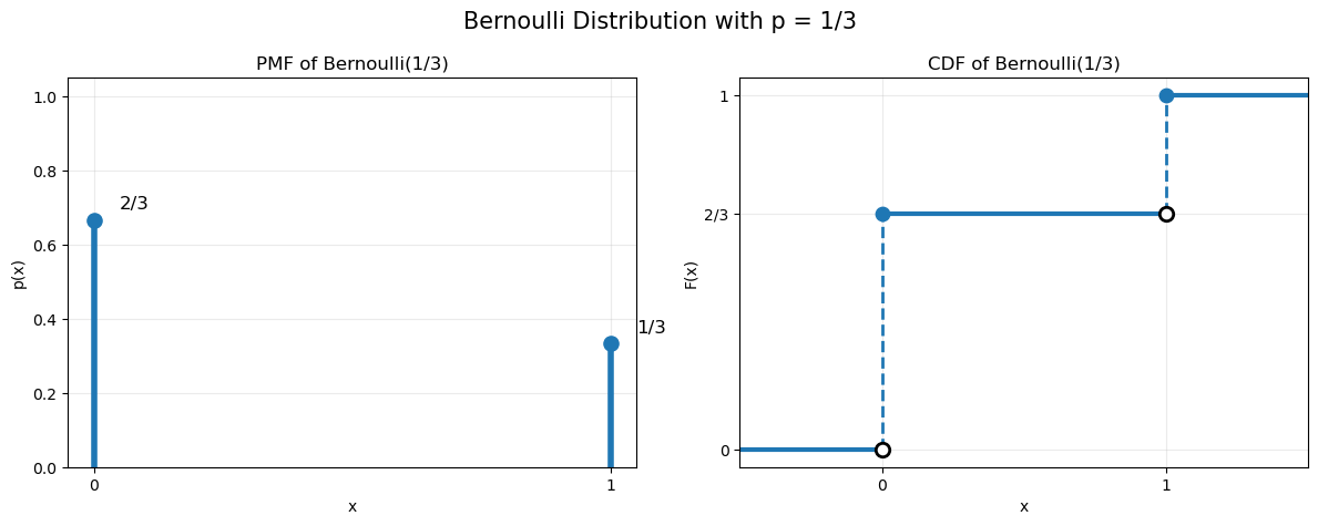
Let \(X\sim\operatorname{Bernoulli}(p)\). Its cumulative distribution function is

\[ F(x)= \begin{cases} 0,&x<0,\\[1ex] 1-p,&0\le x<1,\\[1ex] 1,&x\ge1. \end{cases} \]

Notice that the CDF is a step function with jumps equal to the probabilities of the corresponding outcomes.

import numpy as np
import matplotlib.pyplot as plt

p = 1 / 3

x_values = np.array([0, 1])
pmf = np.array([1 - p, p])

fig, axes = plt.subplots(1, 2, figsize=(12, 4.8))

# =========================
# PMF
# =========================

ax = axes[0]

ax.vlines(x_values, 0, pmf, linewidth=4)
ax.scatter(x_values, pmf, s=90, zorder=3)

ax.set_xticks([0, 1])
ax.set_ylim(0, 1.05)

ax.set_xlabel("x")
ax.set_ylabel("p(x)")
ax.set_title("PMF of Bernoulli(1/3)")

ax.text(0.05, 1 - p + 0.03, "2/3", fontsize=12)
ax.text(1.05, p + 0.03, "1/3", fontsize=12)

ax.grid(alpha=0.25)

# =========================
# CDF
# =========================

ax = axes[1]

# Horizontal pieces of the CDF
ax.hlines(0, -0.5, 0, linewidth=3)
ax.hlines(1 - p, 0, 1, linewidth=3)
ax.hlines(1, 1, 1.5, linewidth=3)

# Open circles: left limits
ax.scatter(
    [0, 1],
    [0, 1 - p],
    s=80,
    facecolors="white",
    edgecolors="black",
    linewidth=2,
    zorder=5
)

# Closed circles: actual CDF values
ax.scatter([0, 1], [1 - p, 1], s=80, zorder=6)

# Vertical jumps
ax.vlines(0, 0, 1 - p, linestyle="--", linewidth=2)
ax.vlines(1, 1 - p, 1, linestyle="--", linewidth=2)

ax.set_xlim(-0.5, 1.5)
ax.set_ylim(-0.05, 1.05)

ax.set_xticks([0, 1])
ax.set_yticks([0, 1 - p, 1])
ax.set_yticklabels(["0", "2/3", "1"])

ax.set_xlabel("x")
ax.set_ylabel("F(x)")
ax.set_title("CDF of Bernoulli(1/3)")

ax.grid(alpha=0.25)

plt.suptitle("Bernoulli Distribution with p = 1/3", fontsize=15)
plt.tight_layout()
plt.show()

2 Continuous Probability Distributions

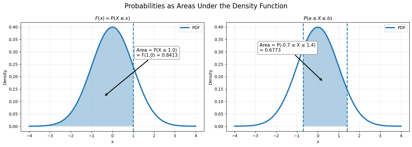
A probability distribution is called absolutely continuous if there exists a non-negative function

\[ p:\mathbb R\rightarrow\mathbb R_+ \]

such that

\[ F(x)=\int_{-\infty}^{x}p(t)\,dt, \qquad x\in\mathbb R. \]

The function \(p(x)\) is called the probability density function (PDF) of the distribution.

import numpy as np
import matplotlib.pyplot as plt
from scipy.stats import uniform, expon, norm

np.random.seed(42)

import numpy as np
import matplotlib.pyplot as plt
from scipy.stats import norm

# Common x-grid
x = np.linspace(-4, 4, 1000)
pdf = norm.pdf(x)

fig, axes = plt.subplots(1, 2, figsize=(14, 5))

# =====================================================
# Left: CDF as accumulated area
# =====================================================

x0 = 1.0
prob1 = norm.cdf(x0)

ax = axes[0]

ax.plot(x, pdf, linewidth=3, label="PDF")

x_fill = x[x <= x0]
pdf_fill = norm.pdf(x_fill)

ax.fill_between(x_fill, pdf_fill, alpha=0.35)

ax.axvline(x0, linestyle="--", linewidth=2)

ax.annotate(
    f"Area = P(X ≤ {x0})\n= F({x0}) = {prob1:.4f}",
    xy=(-0.4, 0.12),
    xytext=(1.15, 0.28),
    fontsize=11,
    arrowprops=dict(arrowstyle="->", lw=2),
    bbox=dict(boxstyle="round,pad=0.4", fc="white", ec="gray")
)

ax.set_title(r"$F(x)=P(X\leq x)$")
ax.set_xlabel("x")
ax.set_ylabel("Density")
ax.grid(alpha=0.25)
ax.legend()

# =====================================================
# Right: Probability on an interval
# =====================================================

a = -0.7
b = 1.4

prob2 = norm.cdf(b) - norm.cdf(a)

ax = axes[1]

ax.plot(x, pdf, linewidth=3, label="PDF")

x_fill = x[(x >= a) & (x <= b)]
pdf_fill = norm.pdf(x_fill)

ax.fill_between(x_fill, pdf_fill, alpha=0.35)

ax.axvline(a, linestyle="--", linewidth=2)
ax.axvline(b, linestyle="--", linewidth=2)

ax.annotate(
    f"Area = P({a} ≤ X ≤ {b})\n= {prob2:.4f}",
    xy=(0.25, 0.18),
    xytext=(-2.8, 0.30),
    fontsize=11,
    arrowprops=dict(arrowstyle="->", lw=2),
    bbox=dict(boxstyle="round,pad=0.4", fc="white", ec="gray")
)

ax.set_title(r"$P(a\leq X\leq b)$")
ax.set_xlabel("x")
ax.set_ylabel("Density")
ax.grid(alpha=0.25)
ax.legend()

plt.suptitle("Probabilities as Areas Under the Density Function", fontsize=16)

plt.tight_layout()
plt.show()

2.1 Properties of the Probability Density Function

1. If the cumulative distribution function is differentiable, then

\[ p(x)=F'(x). \]

2. Every probability density function integrates to one,

\[ \int_{-\infty}^{\infty}p(x)\,dx=1. \]

3. The probability of any Borel set \(B\subseteq\mathbb R\) is obtained by integrating the density over that set,

\[ P(B)=\int_B p(t)\,dt. \]

In particular,

\[ P(a\le X\le b)=\int_a^b p(t)\,dt. \]

2.2 Examples of Absolutely Continuous Distributions

2.2.1 Uniform Distribution

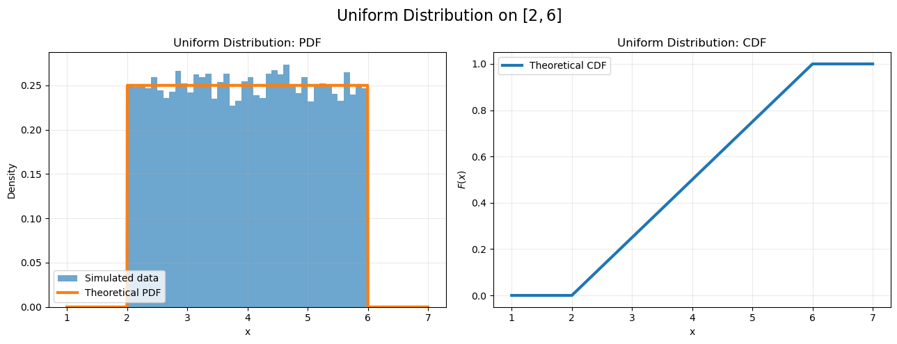
Let $ XU([a,b])$, where \(a<b\). The probability density function is

\[ p(x)= \begin{cases} \dfrac1{b-a},&a\le x\le b,\\[1ex] 0,&\text{otherwise}. \end{cases} \]

Every interval of the same length inside \([a,b]\) has the same probability.

import numpy as np
import matplotlib.pyplot as plt
from scipy.stats import uniform

# Parameters
a = 2
b = 6
n = 20_000

# Simulated sample
sample = np.random.uniform(a, b, size=n)

# Theoretical curves
x = np.linspace(a - 1, b + 1, 1000)
pdf = uniform.pdf(x, loc=a, scale=b - a)
cdf = uniform.cdf(x, loc=a, scale=b - a)

fig, axes = plt.subplots(1, 2, figsize=(13, 5))

# =====================================================
# PDF
# =====================================================

ax = axes[0]

ax.hist(
    sample,
    bins=40,
    density=True,
    alpha=0.65,
    label="Simulated data"
)

ax.plot(
    x,
    pdf,
    linewidth=3,
    label="Theoretical PDF"
)

ax.set_title("Uniform Distribution: PDF")
ax.set_xlabel("x")
ax.set_ylabel("Density")
ax.grid(alpha=0.25)
ax.legend()

# =====================================================
# CDF
# =====================================================

ax = axes[1]

ax.plot(
    x,
    cdf,
    linewidth=3,
    label="Theoretical CDF"
)

ax.set_title("Uniform Distribution: CDF")
ax.set_xlabel("x")
ax.set_ylabel(r"$F(x)$")
ax.set_ylim(-0.05, 1.05)
ax.grid(alpha=0.25)
ax.legend()

plt.suptitle(
    rf"Uniform Distribution on $[{a},{b}]$",
    fontsize=16
)

plt.tight_layout()
plt.show()

2.2.2 Exponential Distribution

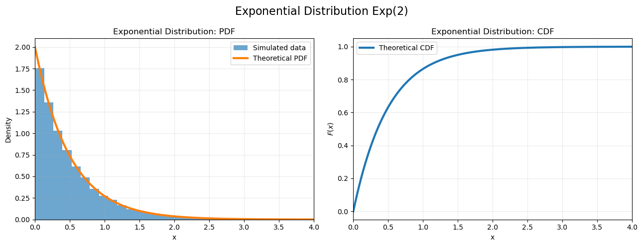
Let \(X\sim\operatorname{Exp}(\lambda)\), where \(\lambda>0\). Its probability density function is

\[ p(x)= \begin{cases} \lambda e^{-\lambda x},&x\ge0,\\[1ex] 0,&x<0. \end{cases} \]

The exponential distribution is commonly used to model waiting times.

import numpy as np
import matplotlib.pyplot as plt
from scipy.stats import expon

# Parameters
lam = 2
n = 20_000

# Simulated sample
sample = np.random.exponential(scale=1/lam, size=n)

# Theoretical curves
x = np.linspace(0, 4, 1000)
pdf = expon.pdf(x, scale=1/lam)
cdf = expon.cdf(x, scale=1/lam)

fig, axes = plt.subplots(1, 2, figsize=(13, 5))

# =====================================================
# PDF
# =====================================================

ax = axes[0]

ax.hist(
    sample,
    bins=40,
    density=True,
    alpha=0.65,
    label="Simulated data"
)

ax.plot(
    x,
    pdf,
    linewidth=3,
    label="Theoretical PDF"
)

ax.set_title(r"Exponential Distribution: PDF")
ax.set_xlabel("x")
ax.set_ylabel("Density")
ax.set_xlim(0, 4)
ax.grid(alpha=0.25)
ax.legend()

# =====================================================
# CDF
# =====================================================

ax = axes[1]

ax.plot(
    x,
    cdf,
    linewidth=3,
    label="Theoretical CDF"
)

ax.set_title(r"Exponential Distribution: CDF")
ax.set_xlabel("x")
ax.set_ylabel(r"$F(x)$")
ax.set_xlim(0, 4)
ax.set_ylim(-0.05, 1.05)
ax.grid(alpha=0.25)
ax.legend()

plt.suptitle(
    r"Exponential Distribution $\mathrm{Exp}(2)$",
    fontsize=16
)

plt.tight_layout()
plt.show()

2.2.3 Normal Distribution

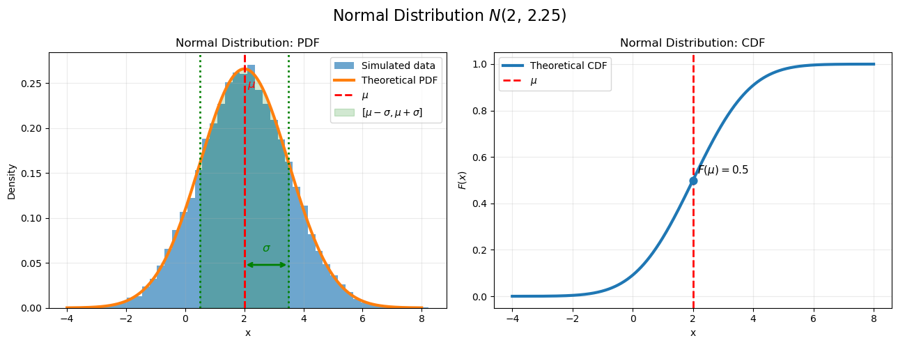
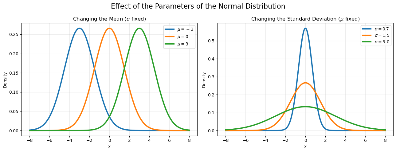
A random variable is said to follow a normal distribution with parameters \(\mu\in\mathbb R\) and \(\sigma^2>0\), if its probability density function is

\[ p(x)= \frac1{\sqrt{2\pi}\sigma} \exp\!\left( -\frac{(x-\mu)^2}{2\sigma^2} \right). \]

We write

\[ \boxed{ X\sim N(\mu,\sigma^2) } \]

import numpy as np
import matplotlib.pyplot as plt
from scipy.stats import norm

# Parameters
mu = 2
sigma = 1.5
n = 20_000

# Simulated sample
sample = np.random.normal(mu, sigma, size=n)

# Theoretical curves
x = np.linspace(mu - 4*sigma, mu + 4*sigma, 1000)
pdf = norm.pdf(x, loc=mu, scale=sigma)
cdf = norm.cdf(x, loc=mu, scale=sigma)

fig, axes = plt.subplots(1, 2, figsize=(13, 5))

# =====================================================
# PDF
# =====================================================

ax = axes[0]

ax.hist(
    sample,
    bins=45,
    density=True,
    alpha=0.65,
    label="Simulated data"
)

ax.plot(
    x,
    pdf,
    linewidth=3,
    label="Theoretical PDF"
)

ax.axvline(
    mu,
    color="red",
    linestyle="--",
    linewidth=2,
    label=r"$\mu$"
)

ax.text(
    mu + 0.1,
    np.max(pdf) * 0.92,
    r"$\mu$",
    color="red",
    fontsize=12
)

# Mean
ax.axvline(
    mu,
    color="red",
    linestyle="--",
    linewidth=2,
    #label=r"$\mu$"
)

# One standard deviation
ax.axvline(
    mu - sigma,
    color="green",
    linestyle=":",
    linewidth=2
)

ax.axvline(
    mu + sigma,
    color="green",
    linestyle=":",
    linewidth=2
)

# Horizontal arrow showing sigma
y_arrow = np.max(pdf) * 0.18

ax.annotate(
    "",
    xy=(mu + sigma, y_arrow),
    xytext=(mu, y_arrow),
    arrowprops=dict(arrowstyle="<->", lw=2, color="green")
)

ax.text(
    mu + sigma/2,
    y_arrow + 0.015,
    r"$\sigma$",
    color="green",
    fontsize=12,
    ha="center"
)

# Shade the interval [mu-sigma, mu+sigma]
x_fill = x[(x >= mu - sigma) & (x <= mu + sigma)]

ax.fill_between(
    x_fill,
    norm.pdf(x_fill, mu, sigma),
    alpha=0.18,
    color="green",
    label=r"$[\mu-\sigma,\mu+\sigma]$"
)
ax.set_title("Normal Distribution: PDF")
ax.set_xlabel("x")
ax.set_ylabel("Density")
ax.grid(alpha=0.25)
ax.legend()

# =====================================================
# CDF
# =====================================================

ax = axes[1]

ax.plot(
    x,
    cdf,
    linewidth=3,
    label="Theoretical CDF"
)

ax.axvline(
    mu,
    color="red",
    linestyle="--",
    linewidth=2,
    label=r"$\mu$"
)

ax.scatter([mu], [0.5], s=60, zorder=5)

ax.text(
    mu + 0.15,
    0.53,
    r"$F(\mu)=0.5$",
    fontsize=11
)

ax.set_title("Normal Distribution: CDF")
ax.set_xlabel("x")
ax.set_ylabel(r"$F(x)$")
ax.set_ylim(-0.05, 1.05)
ax.grid(alpha=0.25)
ax.legend()

plt.suptitle(
    rf"Normal Distribution $N({mu},\,{sigma**2:.2f})$",
    fontsize=16
)

plt.tight_layout()
plt.show()

import numpy as np
import matplotlib.pyplot as plt
from scipy.stats import norm

fig, axes = plt.subplots(1, 2, figsize=(13, 5))

# =====================================================
# Effect of changing the mean
# =====================================================

x = np.linspace(-8, 8, 1000)
sigma = 1.5
mus = [-3, 0, 3]

ax = axes[0]

for mu in mus:
    ax.plot(
        x,
        norm.pdf(x, loc=mu, scale=sigma),
        linewidth=3,
        label=rf"$\mu={mu}$"
    )

ax.set_title(r"Changing the Mean ($\sigma$ fixed)")
ax.set_xlabel("x")
ax.set_ylabel("Density")
ax.grid(alpha=0.25)
ax.legend()

# =====================================================
# Effect of changing the standard deviation
# =====================================================

x = np.linspace(-8, 8, 1000)
mu = 0
sigmas = [0.7, 1.5, 3.0]

ax = axes[1]

for sigma in sigmas:
    ax.plot(
        x,
        norm.pdf(x, loc=mu, scale=sigma),
        linewidth=3,
        label=rf"$\sigma={sigma}$"
    )

ax.set_title(r"Changing the Standard Deviation ($\mu$ fixed)")
ax.set_xlabel("x")
ax.set_ylabel("Density")
ax.grid(alpha=0.25)
ax.legend()

plt.suptitle(
    "Effect of the Parameters of the Normal Distribution",
    fontsize=16
)

plt.tight_layout()
plt.show()

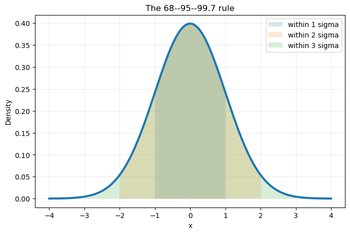
The normal distribution is one of the most important probability distributions in statistics and data science. Many natural phenomena are approximately normally distributed, and many statistical procedures are based on this distribution.

A particularly important special case is the standard normal distribution

\[ N(0,1), \]

which will play a central role throughout the remainder of the course.

2.3 The Standard Normal Table

The cumulative distribution function of the standard normal distribution, \(Z\sim N(0,1)\), is denoted by

\[ \Phi(z)=P(Z\le z). \]

Unlike the cumulative distribution functions of the uniform or exponential distributions, the integral

\[ \Phi(z) = \frac1{\sqrt{2\pi}} \int_{-\infty}^{z} e^{-t^2/2}\,dt \]

cannot be evaluated using elementary functions.

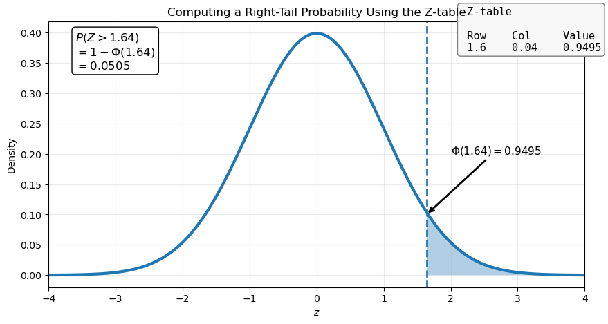
For this reason, values of \(\Phi(z)\) are usually obtained from a standard normal table, often called the Z-table.

2.3.1 How is the Z-table organized?

The Z-table contains numerical values of \(\Phi(z)=P(Z\le z)\) for many values of \(z\).

Typically,

• the row contains the first decimal digit of \(z\);
• the column contains the second decimal digit.

Suppose we want to compute \(P(Z\le1.23)\). Looking up the entry corresponding to row 1.2, and column 0.03, we obtain approximately

\[ \boxed{\Phi(1.23)\approx0.8907.} \]

Therefore,

\[ P(N(0,1)\le1.23)\approx0.8907. \]

import numpy as np
import matplotlib.pyplot as plt
from scipy.stats import norm

# Example
z = 1.64

x = np.linspace(-4, 4, 1000)
pdf = norm.pdf(x)

# Right tail
x_fill = x[x >= z]
pdf_fill = norm.pdf(x_fill)

left_prob = norm.cdf(z)
right_prob = 1 - left_prob

plt.figure(figsize=(10, 5))

# PDF
plt.plot(x, pdf, linewidth=3)
plt.fill_between(x_fill, pdf_fill, alpha=0.35)

plt.axvline(z, linestyle="--", linewidth=2)

# Probability annotation
plt.text(
    -3.6,
    0.34,
    rf"$P(Z>{z})$"
    "\n"
    rf"$=1-\Phi({z})$"
    "\n"
    rf"$={right_prob:.4f}$",
    fontsize=12,
    bbox=dict(boxstyle="round", fc="white")
)

# -------------------------------------------------
# Fake Z-table
# -------------------------------------------------

table_text = (
    " Z-table\n\n"
    " Row    Col     Value\n"
    " 1.6    0.04    0.9495"
)

plt.text(
    2.15,
    0.37,
    table_text,
    fontsize=11,
    family="monospace",
    bbox=dict(boxstyle="round", fc="#F8F8F8", ec="gray")
)

plt.annotate(
    r"$\Phi(1.64)=0.9495$",
    xy=(z, 0.10),
    xytext=(2.0, 0.20),
    arrowprops=dict(arrowstyle="->", lw=2),
    fontsize=11
)

plt.title(r"Computing a Right-Tail Probability Using the Z-table")
plt.xlabel("$z$")
plt.ylabel("Density")
plt.grid(alpha=0.25)

plt.xlim(-4,4)

plt.show()

mu = 0
sigma = 1

x = np.linspace(-4, 4, 1000)
pdf = norm.pdf(x, loc=mu, scale=sigma)

plt.figure(figsize=(8, 5))
plt.plot(x, pdf, linewidth=3)

for k in [1, 2, 3]:
    x_fill = x[(x >= mu - k * sigma) & (x <= mu + k * sigma)]
    plt.fill_between(x_fill, norm.pdf(x_fill), alpha=0.18, label=f"within {k} sigma")

plt.title("The 68--95--99.7 rule")
plt.xlabel("x")
plt.ylabel("Density")
plt.legend()
plt.grid(alpha=0.25)
plt.show()

2.4 Why is the normal distribution so important?

Many real-world variables are approximately normally distributed. Human heights, standardized test scores, measurement errors, IQ scores, and many biological characteristics often follow a distribution that is remarkably close to a normal distribution. Even when the data are not perfectly normal, the normal distribution frequently provides an excellent approximation.

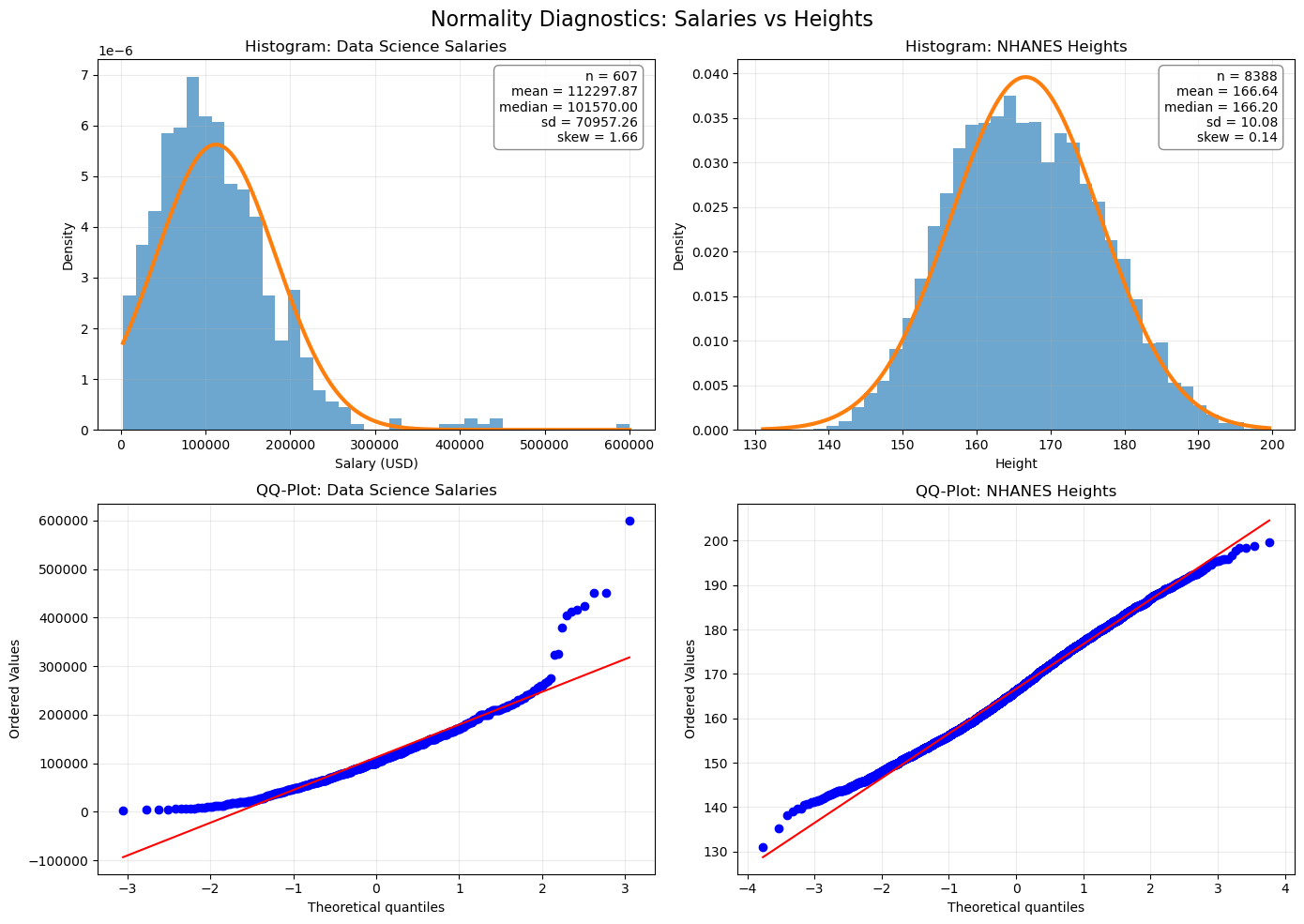
In the examples below, we compare two real datasets:

• Data Science salaries (Worldwide, 2023) — the distribution is noticeably right-skewed because a small number of very highly paid professionals earn much more than the majority.
• NHANES adult heights (United States, 2017–2020) — the distribution is very close to a normal distribution, as predicted by many biological models.

The histograms and QQ-plots clearly illustrate this contrast. While salaries deviate substantially from normality, human heights closely follow a bell-shaped curve, making the normal distribution an excellent model.

This is one of the main reasons why the normal distribution plays such a central role in probability and statistics. In later seminars, we will see that many statistical methods—including confidence intervals, hypothesis tests, linear regression, and the Central Limit Theorem—are built upon the remarkable mathematical properties of the normal distribution.

import numpy as np
import pandas as pd
import matplotlib.pyplot as plt
import scipy.stats as stats

from scipy.stats import norm, skew, kurtosis

# ==========================================================
# 1. Load data
# ==========================================================

salary_df = pd.read_csv("data/ds_salaries.csv")
height_df = pd.read_csv("data/NHANES Weight and Height.csv")

# Salary column
salary_col = [col for col in salary_df.columns if "salary" in col.lower() and "usd" in col.lower()][0]
salary = salary_df[salary_col].dropna()
salary = salary[salary > 0].values

# Height column
height_col = [col for col in height_df.columns if "height" in col.lower()][0]
height = height_df[height_col].dropna()
height = height[height > 0].values

# ==========================================================
# 2. Summary statistics
# ==========================================================

summary = pd.DataFrame({
    "Dataset": [
        "Data science salaries",
        "NHANES heights"
    ],
    "Year": [
        "2023",
        "2017–2020"
    ],
    "Country": [
        "Worldwide",
        "United States"
    ],
    "Sample size": [
        len(salary),
        len(height)
    ],
    "Mean": [
        np.mean(salary),
        np.mean(height)
    ],
    "Median": [
        np.median(salary),
        np.median(height)
    ],
    "Std. deviation": [
        np.std(salary, ddof=1),
        np.std(height, ddof=1)
    ],
    "Skewness": [
        skew(salary),
        skew(height)
    ],
    "Excess kurtosis": [
        kurtosis(salary)
    ,
        kurtosis(height)
    ]
})

display(summary.round({
    "Mean": 2,
    "Median": 2,
    "Std. deviation": 2,
    "Skewness": 2,
    "Excess kurtosis": 2
}))

# ==========================================================
# 3. Histograms and QQ-plots
# ==========================================================

fig, axes = plt.subplots(2, 2, figsize=(14, 10))

datasets = [
    (salary, "Data Science Salaries", "Salary (USD)"),
    (height, "NHANES Heights", "Height")
]

for j, (data, title, xlabel) in enumerate(datasets):
    
    mu_hat = np.mean(data)
    sigma_hat = np.std(data, ddof=1)
    
    x_grid = np.linspace(np.min(data), np.max(data), 500)
    normal_density = norm.pdf(x_grid, loc=mu_hat, scale=sigma_hat)
    
    # Histogram
    ax = axes[0, j]
    
    ax.hist(
        data,
        bins=40,
        density=True,
        alpha=0.65,
        #label="Observed data"
    )
    
    ax.plot(
        x_grid,
        normal_density,
        linewidth=3,
        #label="Fitted normal density"
    )
    
    ax.set_title(f"Histogram: {title}")
    ax.set_xlabel(xlabel)
    ax.set_ylabel("Density")
    ax.grid(alpha=0.25)
    #ax.legend()
    
    text = (
        f"n = {len(data)}\n"
        f"mean = {mu_hat:.2f}\n"
        f"median = {np.median(data):.2f}\n"
        f"sd = {sigma_hat:.2f}\n"
        f"skew = {skew(data):.2f}"
    )
    
    ax.text(
    0.97,
    0.97,
    text,
    transform=ax.transAxes,
    ha="right",
    va="top",
    fontsize=10,
    bbox=dict(
        boxstyle="round,pad=0.4",
        facecolor="white",
        edgecolor="gray",
        alpha=0.9
    )
)
    
    # QQ-plot
    ax = axes[1, j]
    
    stats.probplot(data, dist="norm", plot=ax)
    
    ax.set_title(f"QQ-Plot: {title}")
    ax.grid(alpha=0.25)

plt.suptitle(
    "Normality Diagnostics: Salaries vs Heights",
    fontsize=16
)

plt.tight_layout()
plt.show()

	Dataset	Year	Country	Sample size	Mean	Median	Std. deviation	Skewness	Excess kurtosis
0	Data science salaries	2023	Worldwide	607	112297.87	101570.0	70957.26	1.66	6.29
1	NHANES heights	2017–2020	United States	8388	166.64	166.2	10.08	0.14	-0.42

3 Simulating Random Variables from Uniform Random Numbers

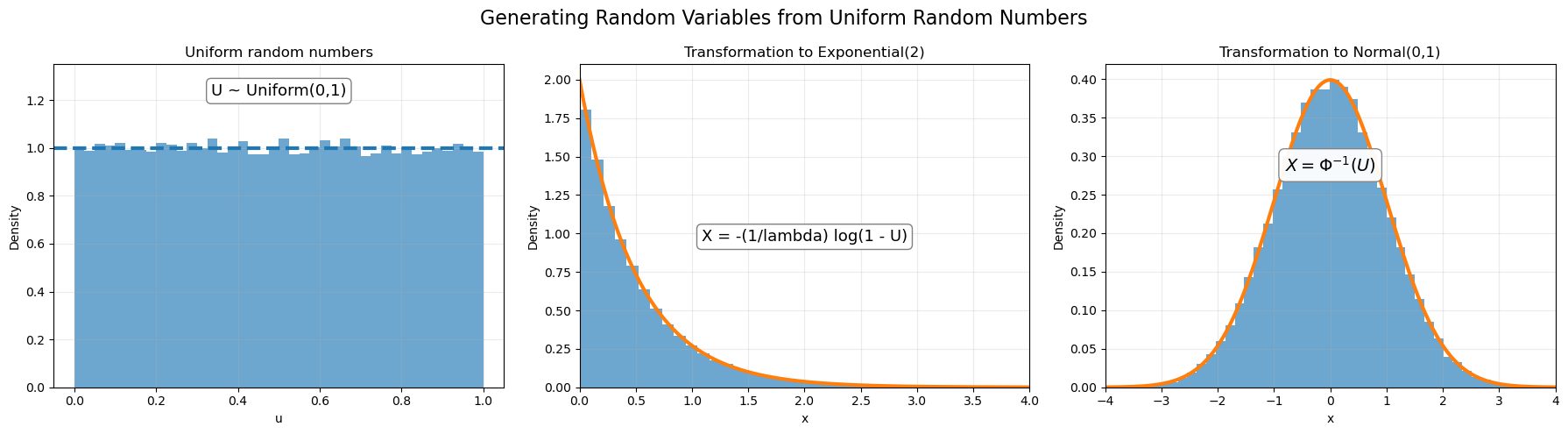
Computers do not directly generate random variables from every possible distribution. In practice, the basic object generated by a computer is usually a number that behaves like

\[ U\sim U(0,1). \]

From this uniform random variable, we can generate random variables with many other distributions by applying a suitable function.

The key idea is the inverse transform method.

3.1 The Inverse Transform Method

Let \(U\sim U(0,1)\) and let \(F\) be the CDF of a continuous random variable. Define

\[ X=F^{-1}(U). \]

Then \(X\) has CDF \(F\). Indeed, for any \(x\),

\[ P(X\le x) = P(F^{-1}(U)\le x) = P(U\le F(x)) = F(x), \]

because \(U\) is uniformly distributed on \([0,1]\).

Thus, \(X=F^{-1}(U)\) transforms uniform random numbers into random numbers with distribution function \(F\).

3.2 Example: Exponential Distribution

Let \(X\sim \operatorname{Exp}(\lambda)\). Its cumulative distribution function is

\[ F(x)=1-e^{-\lambda x}, \qquad x\ge0. \]

To generate \(X\), we solve \(u=1-e^{-\lambda x}\) for \(x\).

This gives

\[ x=-\frac1\lambda\ln(1-u). \]

Hence, if \(U\sim U(0,1)\), then

\[ \boxed{ X=-\frac1\lambda\ln(1-U) \sim \operatorname{Exp}(\lambda). } \]

Since \(1-U\) has the same distribution as \(U\), we often write simply \(X=-\frac1\lambda\ln U\).

import numpy as np
import matplotlib.pyplot as plt
from scipy.stats import expon, norm

np.random.seed(42)

n = 50000
lam = 2

# Uniform random numbers
U = np.random.uniform(0, 1, size=n)

# Transformations
X_exp = -(1 / lam) * np.log(1 - U)
X_norm = norm.ppf(U)

# Theoretical densities
x_exp = np.linspace(0, 4, 1000)
pdf_exp = expon.pdf(x_exp, scale=1 / lam)

x_norm = np.linspace(-4, 4, 1000)
pdf_norm = norm.pdf(x_norm)

fig, axes = plt.subplots(1, 3, figsize=(18, 5))

# Uniform
ax = axes[0]
ax.hist(U, bins=40, density=True, alpha=0.65)
ax.axhline(1, linestyle="--", linewidth=3)
ax.set_title("Uniform random numbers")
ax.text(
    0.5, 1.22,
    "U ~ Uniform(0,1)",
    ha="center",
    fontsize=13,
    bbox=dict(boxstyle="round", facecolor="white", edgecolor="gray")
)
ax.set_xlabel("u")
ax.set_ylabel("Density")
ax.set_ylim(0, 1.35)
ax.grid(alpha=0.25)

# Exponential
ax = axes[1]
ax.hist(X_exp, bins=50, density=True, alpha=0.65)
ax.plot(x_exp, pdf_exp, linewidth=3)
ax.set_title("Transformation to Exponential(2)")
ax.text(
    2.0, 0.95,
    "X = -(1/lambda) log(1 - U)",
    ha="center",
    fontsize=13,
    bbox=dict(boxstyle="round", facecolor="white", edgecolor="gray")
)
ax.set_xlim(0, 4)
ax.set_xlabel("x")
ax.set_ylabel("Density")
ax.grid(alpha=0.25)

# Normal
ax = axes[2]
ax.hist(X_norm, bins=50, density=True, alpha=0.65)
ax.plot(x_norm, pdf_norm, linewidth=3)
ax.set_title("Transformation to Normal(0,1)")
ax.text(
    0,
    0.28,
    r"$X=\Phi^{-1}(U)$",
    ha="center",
    fontsize=14,
    bbox=dict(boxstyle="round,pad=0.35",
              facecolor="white",
              edgecolor="gray",
              alpha=0.95)
)
ax.set_xlim(-4, 4)
ax.set_xlabel("x")
ax.set_ylabel("Density")
ax.grid(alpha=0.25)

plt.suptitle(
    "Generating Random Variables from Uniform Random Numbers",
    fontsize=16
)

plt.tight_layout()
plt.show()