Seminar 4: Discrete Random Variables

1 Probability Distributions and Random Variables

In the previous lectures, probabilities were assigned directly to events in a probability space \((\Omega,\mathcal F,P)\). In practice, however, we are often interested in numerical quantities associated with the outcomes of an experiment, such as the number of heads obtained when tossing a coin several times, the number of customers arriving at a store during one hour, or the height of a randomly selected individual.

Such quantities are modeled by random variables. To study them, we first introduce probability distributions on the real line.

1.1 Borel \(\sigma\)-Algebra

The Borel \(\sigma\)-algebra on \(\mathbb R\), denoted by \(\mathcal B(\mathbb R)\), is the smallest \(\sigma\)-algebra containing all open subsets of \(\mathbb R\).

Elements of \(\mathcal B(\mathbb R)\) are called Borel sets. In particular, every open interval, closed interval, half-open interval, countable union, countable intersection, and complement of such sets belongs to \(\mathcal B(\mathbb R)\).

1.2 Measurable Functions and Random Variables

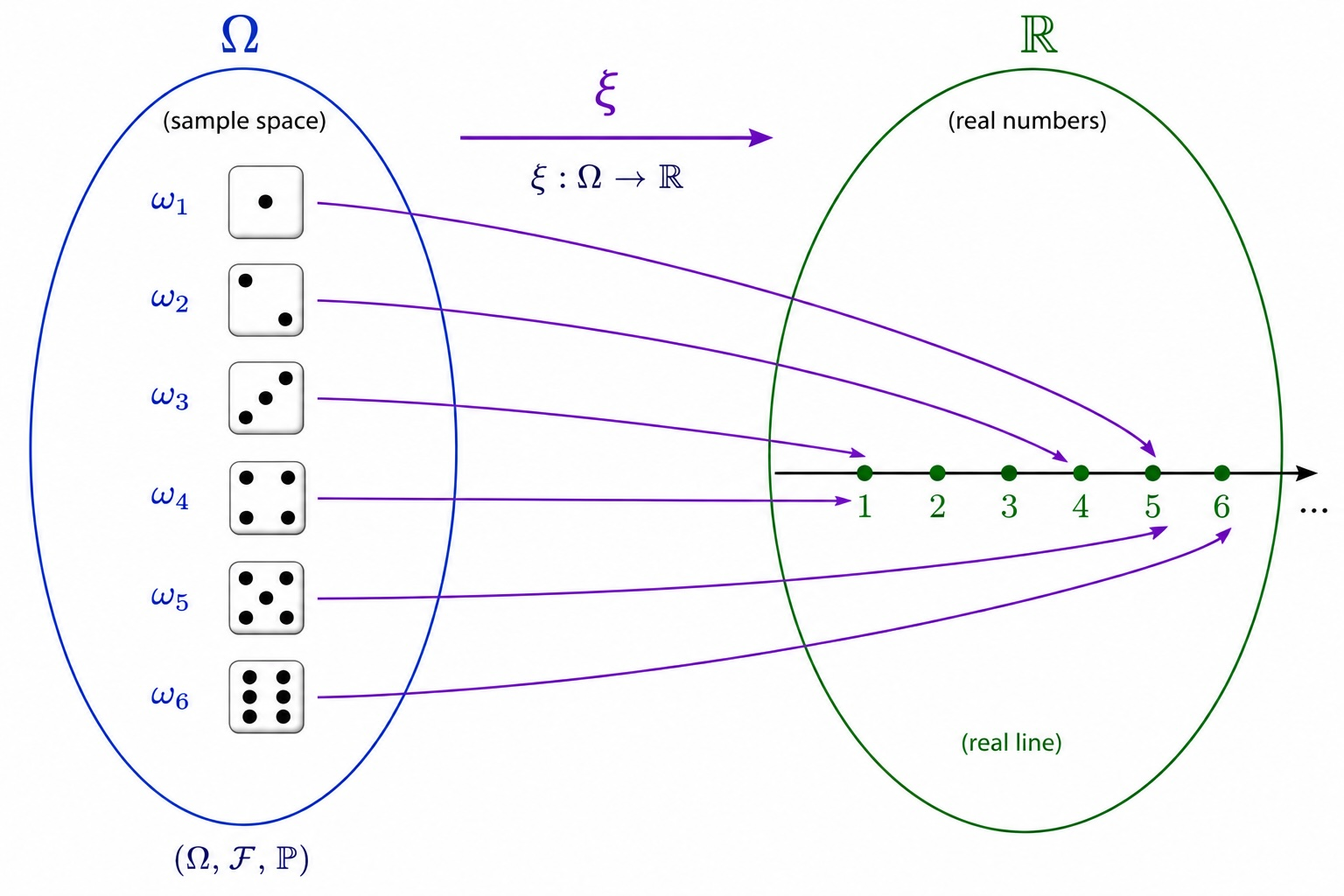
Let \((\Omega,\mathcal F)\) and \((\mathbb R,\mathcal B(\mathbb R))\) be measurable spaces. A function

\[ \xi:\Omega\to\mathbb R \]

is called measurable if

\[ \xi^{-1}(B) = \{\omega\in\Omega:\xi(\omega)\in B\} \in\mathcal F \qquad \forall B\in\mathcal B(\mathbb R). \]

A random variable on a probability space \((\Omega,\mathcal F,P)\) is simply a measurable function \(\xi:\Omega\to\mathbb R\).

We denote by

\[ X_\xi=\{\xi(\omega):\omega\in\Omega\} \]

the set of all possible values of \(\xi\).

If \(X_\xi\) is finite or countable, then \(\xi\) is called a discrete random variable.

1.3 Probability Distributions

A probability distribution is any probability measure on \((\mathbb R,\mathcal B(\mathbb R))\).

That is,

\[ P:\mathcal B(\mathbb R)\to[0,1]. \]

If there exists a finite or countable set \(X\subseteq\mathbb R\) such that \(P(X)=1\), then \(P\) is called a discrete probability distribution.

1.4 Distribution of a Random Variable

Let \(\xi\) be a random variable on \((\Omega,\mathcal F,P)\).

The probability distribution of \(\xi\) is the probability measure \(P_\xi\) on \((\mathbb R,\mathcal B(\mathbb R))\) defined by

\[ P_\xi(B) = P(\{\omega\in\Omega:\xi(\omega)\in B\}) = P(\xi\in B), \qquad B\in\mathcal B(\mathbb R). \]

Thus, the distribution of a random variable completely describes the probabilities of all events involving its values.

1.5 Probability Mass Function (PMF)

Let \(\xi\) be a discrete random variable and let \(X_\xi=\{x_1,x_2,\ldots\}\).

The probability mass function (PMF) of \(\xi\) is the function

\[ p_\xi:\mathbb R\to[0,1] \]

defined by

\[ p_\xi(x_k) = P(\xi=x_k), \qquad x_k\in X_\xi, \]

and $ p_(x)=0$, \(x\notin X_\xi\)

The PMF completely determines the distribution of a discrete random variable and satisfies \(\sum_{x\in X_\xi} p_\xi(x)=1\).

2 Examples of Discrete Probability Distributions

2.1 Uniform Distribution

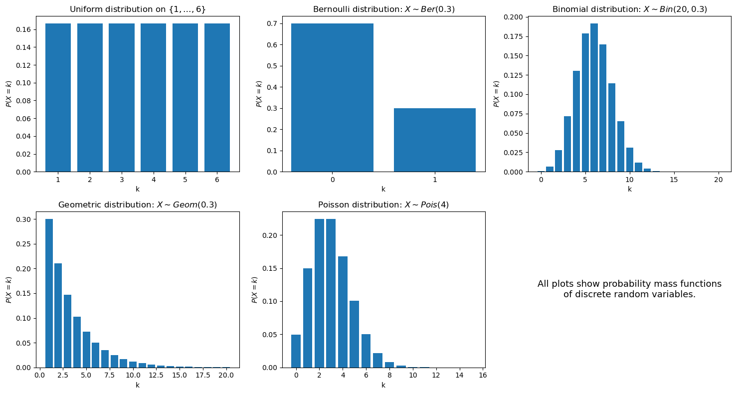
Let \(X\) be a finite set. The uniform distribution on \(X\) is defined by

\[ P(x)=\frac1{|X|}, \qquad x\in X. \]

2.2 Bernoulli Distribution

For \(p\in(0,1)\), \(X=\{0,1\}\), and

\[ P(0)=1-p, \qquad P(1)=p. \]

We write

\[ \xi\sim\operatorname{Ber}(p). \]

2.3 Binomial Distribution

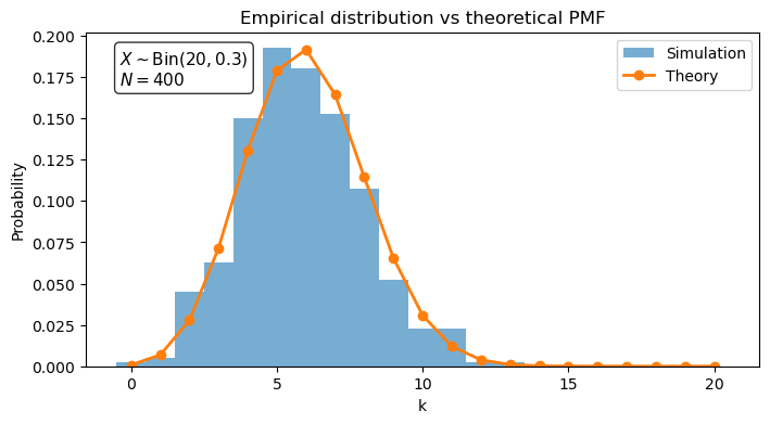
For \(n\in\mathbb N\) and \(p\in(0,1)\), \(X=\{0,1,\ldots,n\}\), and

\[ P(k) = \binom nk p^k(1-p)^{n-k}. \]

We write

\[ \xi\sim\operatorname{Bin}(n,p). \]

2.4 Geometric Distribution

For \(p\in(0,1)\), \(X=\mathbb N \setminus \{0\}\), and

\[ P(k) = (1-p)^{k-1}p, \qquad k\ge1. \]

We write

\[ \xi\sim\operatorname{Geom}(p). \]

2.5 Poisson Distribution

For \(\lambda>0\), \(X=\{0,1,2,\ldots\}\), and

\[ P(k) = \frac{\lambda^k e^{-\lambda}}{k!}. \]

We write

\[ \xi\sim\operatorname{Pois}(\lambda). \]

import numpy as np
import matplotlib.pyplot as plt
from math import comb, factorial, exp

fig, axes = plt.subplots(2, 3, figsize=(15, 8))
axes = axes.ravel()

# 1. Uniform distribution
X = np.arange(1, 7)
pmf = np.ones(len(X)) / len(X)

axes[0].bar(X, pmf)
axes[0].set_title(r"Uniform distribution on $\{1,\ldots,6\}$")
axes[0].set_xlabel("k")
axes[0].set_ylabel(r"$P(X=k)$")

# 2. Bernoulli distribution
p = 0.3
X = np.array([0, 1])
pmf = np.array([1 - p, p])

axes[1].bar(X, pmf)
axes[1].set_title(r"Bernoulli distribution: $X\sim Ber(0.3)$")
axes[1].set_xlabel("k")
axes[1].set_ylabel(r"$P(X=k)$")
axes[1].set_xticks([0, 1])

# 3. Binomial distribution
n, p = 20, 0.3
X = np.arange(n + 1)
pmf = np.array([comb(n, k) * p**k * (1-p)**(n-k) for k in X])

axes[2].bar(X, pmf)
axes[2].set_title(r"Binomial distribution: $X\sim Bin(20,0.3)$")
axes[2].set_xlabel("k")
axes[2].set_ylabel(r"$P(X=k)$")

# 4. Geometric distribution
p = 0.3
X = np.arange(1, 21)
pmf = np.array([(1-p)**(k-1) * p for k in X])

axes[3].bar(X, pmf)
axes[3].set_title(r"Geometric distribution: $X\sim Geom(0.3)$")
axes[3].set_xlabel("k")
axes[3].set_ylabel(r"$P(X=k)$")

# 5. Poisson distribution
lam = 3
X = np.arange(0, 16)
pmf = np.array([lam**k * exp(-lam) / factorial(k) for k in X])

axes[4].bar(X, pmf)
axes[4].set_title(r"Poisson distribution: $X\sim Pois(4)$")
axes[4].set_xlabel("k")
axes[4].set_ylabel(r"$P(X=k)$")

# 6. Empty / optional note
axes[5].axis("off")
axes[5].text(
    0.5, 0.5,
    "All plots show probability mass functions\nof discrete random variables.",
    ha="center",
    va="center",
    fontsize=13
)

plt.tight_layout()
plt.show()

import numpy as np
import matplotlib.pyplot as plt
from math import comb

n, p = 20, 0.3
N = 400

sample = np.random.binomial(n, p, size=N)

x = np.arange(n + 1)
theory = [comb(n, k) * p**k * (1-p)**(n-k) for k in x]

plt.figure(figsize=(8,4))

plt.hist(
    sample,
    bins=np.arange(n+2)-0.5,
    density=True,
    alpha=0.6,
    label="Simulation"
)

plt.plot(
    x,
    theory,
    "o-",
    linewidth=2,
    label="Theory"
)

info = (
    r"$X \sim \mathrm{Bin}(20,0.3)$" "\n"
    rf"$N = {N:,}$"
)

ax = plt.gca()

ax.text(
    0.05,
    0.95,
    rf"$X\sim\mathrm{{Bin}}({n},{p})$" + "\n" + rf"$N={N:,}$",
    transform=ax.transAxes,
    fontsize=11,
    verticalalignment="top",
    bbox=dict(boxstyle="round", facecolor="white", alpha=0.8)
)

plt.xlabel("k")
plt.ylabel("Probability")
plt.title("Empirical distribution vs theoretical PMF")
plt.legend()
plt.show()

3 Poisson Limit Theorem

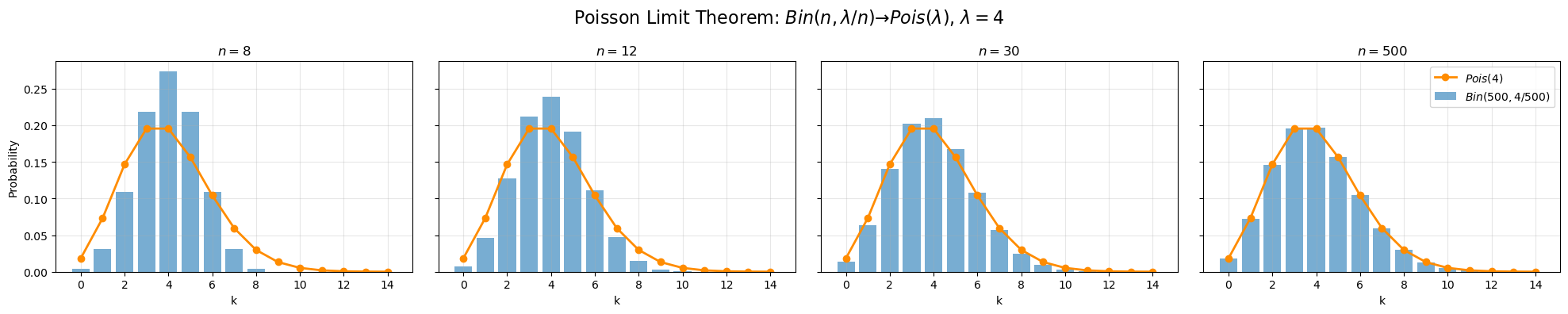
Let \(\xi_n\sim\operatorname{Bin}(n,p_n)\) and suppose that \(np_n\to\lambda>0\).

Then for every fixed \(k\ge0\),

\[ P(\xi_n=k) \longrightarrow \frac{\lambda^k e^{-\lambda}}{k!}. \]

In other words, the binomial distribution converges to the Poisson distribution when the number of trials becomes large and the success probability becomes small in such a way that the expected number of successes remains approximately constant.

import numpy as np
import matplotlib.pyplot as plt
from math import comb, factorial, exp

lambda_ = 4
ns = [8, 12, 30, 500]
x = np.arange(0, 15)

pois = np.array([
    lambda_**k * exp(-lambda_) / factorial(k)
    for k in x
])

fig, axes = plt.subplots(1, 4, figsize=(20, 4), sharey=True)

for ax, n in zip(axes, ns):

    p = lambda_ / n

    binom = np.array([
        comb(n, k) * p**k * (1-p)**(n-k)
        for k in x
    ])

    # Binomial distribution (bars)
    ax.bar(
        x,
        binom,
        alpha=0.6,
        label=fr"$Bin({n},{lambda_}/{n})$"
    )

    # Poisson distribution (line)
    ax.plot(
        x,
        pois,
        "o-",
        color="darkorange",
        linewidth=2,
        label=fr"$Pois({lambda_})$"
    )

    ax.set_title(fr"$n={n}$")
    ax.set_xlabel("k")
    ax.grid(alpha=0.3)

axes[0].set_ylabel("Probability")

fig.suptitle(
    rf"Poisson Limit Theorem: $Bin(n,\lambda/n)\to Pois(\lambda)$, $\lambda={lambda_}$",
    fontsize=16
)

axes[-1].legend(loc="upper right")

plt.tight_layout()
plt.show()

4 Independence of Random Variables

Two discrete random variables \(\xi\) and \(\eta\) are called independent if

\[ P(\xi=x,\eta=y) = P(\xi=x)P(\eta=y) \]

for all possible values \(x\in X_\xi\) and \(y\in X_\eta\).

Similarly, a collection of random variables \(\xi_1,\ldots,\xi_n\) is called mutually independent if

\[ P(\xi_{i_1}=x_{i_1},\ldots,\xi_{i_k}=x_{i_k}) = \prod_{j=1}^{k} P(\xi_{i_j}=x_{i_j}) \]

for every subset \(\{i_1,\ldots,i_k\}\subseteq\{1,\ldots,n\}\).

4.1 Convolution of Discrete Distributions

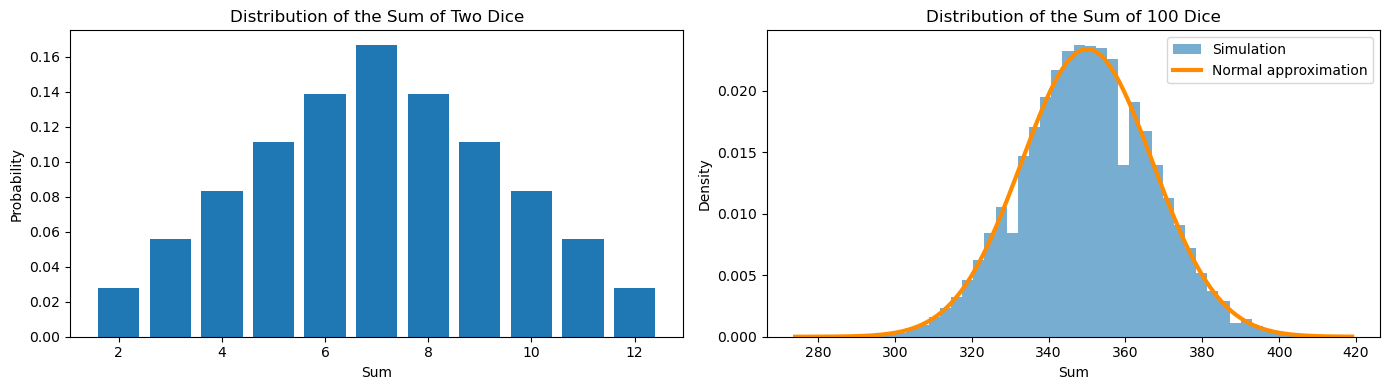
Let \(\xi\) and \(\eta\) be independent discrete random variables. Then

\[ P(\xi+\eta=k) = \sum_{i=-\infty}^{+\infty} P(\xi=i)P(\eta=k-i). \]

This formula is called the convolution formula.

Important examples:

• If \(\xi\sim\operatorname{Bin}(n,p)\) and \(\eta\sim\operatorname{Bin}(m,p)\) are independent, then

\[ \xi+\eta\sim\operatorname{Bin}(n+m,p). \]

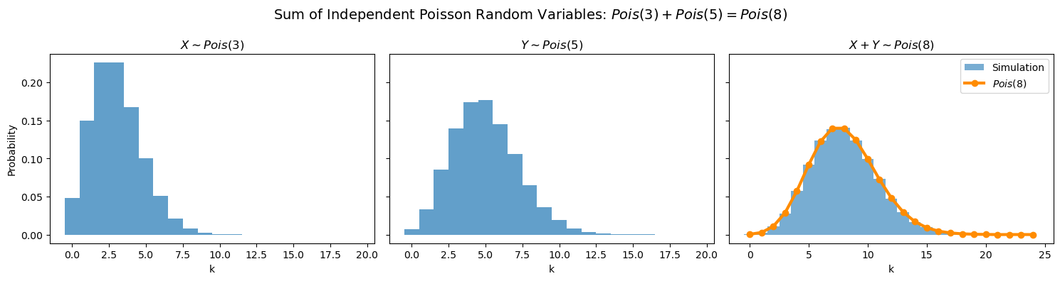
• If \(\xi\sim\operatorname{Pois}(\lambda_1)\) and \(\eta\sim\operatorname{Pois}(\lambda_2)\) are independent, then

\[ \xi+\eta\sim\operatorname{Pois}(\lambda_1+\lambda_2). \]

import numpy as np
import matplotlib.pyplot as plt

np.random.seed(42)

# =====================================================
# Sum of 2 dice (exact distribution)
# =====================================================

die = np.ones(6) / 6
conv = np.convolve(die, die)

sums2 = np.arange(2, 13)

# =====================================================
# Sum of 100 dice (simulation)
# =====================================================

N = 100_000

sample100 = np.random.randint(
    1, 7,
    size=(N, 100)
).sum(axis=1)

# =====================================================
# Normal approximation
# =====================================================

mu = 100 * 3.5
sigma = np.sqrt(100 * 35 / 12)

x = np.linspace(
    sample100.min(),
    sample100.max(),
    1000
)

normal_pdf = (
    1 / (sigma * np.sqrt(2 * np.pi))
    * np.exp(-(x - mu) ** 2 / (2 * sigma ** 2))
)

# =====================================================
# Plot
# =====================================================

fig, axes = plt.subplots(1, 2, figsize=(14, 4))

# Left panel
axes[0].bar(sums2, conv)
axes[0].set_title("Distribution of the Sum of Two Dice")
axes[0].set_xlabel("Sum")
axes[0].set_ylabel("Probability")

# Right panel
axes[1].hist(
    sample100,
    bins=50,
    density=True,
    alpha=0.6,
    label="Simulation"
)

axes[1].plot(
    x,
    normal_pdf,
    color="darkorange",
    linewidth=3,
    label="Normal approximation"
)

axes[1].set_title("Distribution of the Sum of 100 Dice")
axes[1].set_xlabel("Sum")
axes[1].set_ylabel("Density")
axes[1].legend()

plt.tight_layout()
plt.show()

import numpy as np
import matplotlib.pyplot as plt
from math import factorial, exp

np.random.seed(42)

# =====================================================
# Parameters
# =====================================================

lambda1 = 3
lambda2 = 5

N = 100_000

# =====================================================
# Simulation
# =====================================================

X = np.random.poisson(lambda1, size=N)
Y = np.random.poisson(lambda2, size=N)

Z = X + Y

# =====================================================
# Theoretical distribution
# =====================================================

lam = lambda1 + lambda2

k = np.arange(0, 25)

pois_theory = np.array([
    exp(-lam) * lam**i / factorial(i)
    for i in k
])

# =====================================================
# Plot
# =====================================================

fig, axes = plt.subplots(1, 3, figsize=(15, 4), sharey=True)

# X ~ Pois(lambda1)

axes[0].hist(
    X,
    bins=np.arange(-0.5, 20.5, 1),
    density=True,
    alpha=0.7
)

axes[0].set_title(rf"$X\sim Pois({lambda1})$")
axes[0].set_xlabel("k")
axes[0].set_ylabel("Probability")

# Y ~ Pois(lambda2)

axes[1].hist(
    Y,
    bins=np.arange(-0.5, 20.5, 1),
    density=True,
    alpha=0.7
)

axes[1].set_title(rf"$Y\sim Pois({lambda2})$")
axes[1].set_xlabel("k")

# X + Y

axes[2].hist(
    Z,
    bins=np.arange(-0.5, 25.5, 1),
    density=True,
    alpha=0.6,
    label="Simulation"
)

axes[2].plot(
    k,
    pois_theory,
    "o-",
    color="darkorange",
    linewidth=3,
    markersize=6,
    label=rf"$Pois({lam})$"
)

axes[2].set_title(
    rf"$X+Y\sim Pois({lam})$"
)

axes[2].set_xlabel("k")
axes[2].legend()

fig.suptitle(
    rf"Sum of Independent Poisson Random Variables: "
    rf"$Pois({lambda1})+Pois({lambda2})=Pois({lam})$",
    fontsize=14
)

plt.tight_layout()
plt.show()

5 Discrete Random Vectors

So far we have studied a single random variable \(\xi:\Omega\to\mathbb R\). In many applications, however, several random quantities are observed simultaneously. This leads to the notion of a random vector.

5.1 Definition

A 2-dimensional discrete random vector is a pair of discrete random variables

\[ (\xi,\eta). \]

More generally,

\[ (\xi_1,\xi_2,\dots,\xi_n). \]

For every outcome \(\omega\in\Omega\), the random vector assigns a point

\[ (\xi_1(\omega),\xi_2(\omega),\dots,\xi_n(\omega)) \in\mathbb R^n. \]

The set of all possible values is called the support of the random vector.

5.2 Joint Probability Mass Function

The probability distribution of a discrete random vector is described by its joint probability mass function (joint PMF).

5.2.1 Definition

For a discrete random vector \((\xi,\eta)\),

\[ p_{\xi,\eta}(x,y) = \mathbb P(\xi=x,\eta=y). \]

The value \(p_{\xi,\eta}(x,y)\) is the probability that both events occur simultaneously.

The joint PMF satisfies \(p_{\xi,\eta}(x,y)\ge0\), and

\[ \sum_x\sum_y p_{\xi,\eta}(x,y)=1. \]

5.3 Joint PMF Tables

A convenient way to represent a joint PMF is by a table.

5.3.1 Example: Two Fair Dice

For two independent fair dice,

\[ p_{\xi,\eta}(x,y)=\frac1{36}, \qquad x,y\in\{1,\dots,6\}. \]

\[ \begin{array}{c|cccccc} \xi\backslash\eta &1&2&3&4&5&6\\ \hline 1&\frac1{36}&\frac1{36}&\frac1{36}&\frac1{36}&\frac1{36}&\frac1{36}\\ 2&\frac1{36}&\frac1{36}&\frac1{36}&\frac1{36}&\frac1{36}&\frac1{36}\\ 3&\frac1{36}&\frac1{36}&\frac1{36}&\frac1{36}&\frac1{36}&\frac1{36}\\ 4&\frac1{36}&\frac1{36}&\frac1{36}&\frac1{36}&\frac1{36}&\frac1{36}\\ 5&\frac1{36}&\frac1{36}&\frac1{36}&\frac1{36}&\frac1{36}&\frac1{36}\\ 6&\frac1{36}&\frac1{36}&\frac1{36}&\frac1{36}&\frac1{36}&\frac1{36} \end{array} \]

Every cell corresponds to one outcome \((x,y)\).

The sum of all entries of the table must be equal to \(1\).

6 Marginal Distributions

The distributions of \(\xi\) and \(\eta\) can be recovered from the joint PMF.

6.1 Definition

The marginal PMF of \(\xi\) is

\[ p_\xi(x) = \sum_y p_{\xi,\eta}(x,y). \]

Similarly,

\[ p_\eta(y) = \sum_x p_{\xi,\eta}(x,y). \]

In words, we sum over all possible values of the other variable.

6.1.1 Example

For two fair dice,

\[ p_\xi(x) = \sum_{y=1}^{6}\frac1{36} = \frac16. \]

6.2 Independence

The notion of independence extends naturally to random vectors.

6.2.1 Definition

Random variables \(\xi\) and \(\eta\) are independent if

\[ p_{\xi,\eta}(x,y) = p_\xi(x)p_\eta(y) \qquad \forall x,y. \]

Thus, the probability of a pair of outcomes factors into the product of the marginal probabilities.

7 Discrete distributions in ML

7.1 Logistic Regression

Many machine learning problems involve predicting a binary outcome.

Suppose

\[ Y= \begin{cases} 1,& \text{success},\\ 0,& \text{failure}. \end{cases} \]

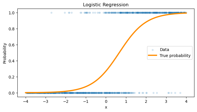
Then

\[ Y\sim Ber(p), \]

where \(p\) is the probability of success. Logistic regression is used when the response variable has only two possible outcomes.

Examples include:

• Will a customer purchase a product?
• Will a student pass an exam?
• Will a patient develop a disease?
• Is an email spam or not spam?
• Will a user click on an advertisement?

In logistic regression, this probability depends on explanatory variables. For example, an online store may use

\[ (x_1,x_2,x_3) = (\text{age},\text{income},\text{number of previous purchases}) \]

to predict the probability that a customer makes a purchase.

For a single feature \(x\), the model assumes

\[ p(x) = \frac{1}{1+e^{-(\beta_0+\beta_1 x)}}. \]

Thus,

\[ Y\mid x \sim Ber(p(x)). \]

Logistic regression is one of the most widely used classification methods in machine learning.

import numpy as np
import matplotlib.pyplot as plt

np.random.seed(42)

n = 1000

x = np.random.uniform(-4, 4, n)

beta0 = -1
beta1 = 1.5

p = 1 / (1 + np.exp(-(beta0 + beta1 * x)))

y = np.random.binomial(1, p)

x_grid = np.linspace(-4, 4, 500)
p_grid = 1 / (1 + np.exp(-(beta0 + beta1 * x_grid)))

plt.figure(figsize=(8,4))

plt.scatter(
    x,
    y,
    alpha=0.15,
    s=15,
    label="Data"
)

plt.plot(
    x_grid,
    p_grid,
    color="darkorange",
    linewidth=3,
    label="True probability"
)

plt.xlabel("x")
plt.ylabel("Probability")
plt.title("Logistic Regression")
plt.legend()

plt.show()

7.2 Poisson Regression

Many applications involve predicting counts.

Examples include:

• number of website visits;
• number of accidents;
• number of insurance claims;
• number of emails received.

In such situations, it is natural to assume

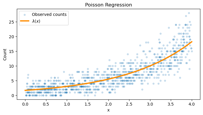
\[ Y\sim Pois(\lambda), \]

where \(\lambda\) is the expected count.

Poisson regression models the parameter \(\lambda\) as

\[ \lambda(x) = e^{\beta_0+\beta_1 x}. \]

The exponential function guarantees that \(\lambda(x)>0\).

For example, a company may use

\[ (x_1,x_2,x_3) = (\text{advertising budget}, \text{season}, \text{number of users}) \]

to predict the expected number of website visits. Thus,

\[ Y\mid x \sim Pois(\lambda(x)). \]

Poisson regression is one of the most important generalized linear models.

import numpy as np
import matplotlib.pyplot as plt

np.random.seed(42)

n = 1000

x = np.random.uniform(0, 4, n)

beta0 = 0.5
beta1 = 0.6

lam = np.exp(beta0 + beta1 * x)

y = np.random.poisson(lam)

x_grid = np.linspace(0, 4, 500)
lam_grid = np.exp(beta0 + beta1 * x_grid)

plt.figure(figsize=(8,4))

plt.scatter(
    x,
    y,
    alpha=0.2,
    s=15,
    label="Observed counts"
)

plt.plot(
    x_grid,
    lam_grid,
    color="darkorange",
    linewidth=3,
    label=r"$\lambda(x)$"
)

plt.xlabel("x")
plt.ylabel("Count")
plt.title("Poisson Regression")
plt.legend()

plt.show()